UnivariateSplinewithUnits

class interpolated_coordinates.utils.spline.UnivariateSplinewithUnits(x: Quantity, y: Quantity, w: ndarray | None = None, bbox: BBoxType = [None, None], k: int = 3, s: float | None = None, ext: int | str | None = 0, check_finite: bool = False, *, x_unit: UnitLikeType | None = None, y_unit: UnitLikeType | None = None)

Bases: UnivariateSpline

1-D smoothing spline fit to a given set of data points.

Fits a spline y = spl(x) of degree k to the provided x, y data. s specifies the number of knots by specifying a smoothing condition.

Parameters:

x(N,) Quantity-like or array_like

1-D array of independent input data. Must be increasing; must be strictly increasing if s is 0.

y(N,) Quantity-like or array_like

1-D array of dependent input data, of the same length as x.

w(N,) array_like, optional

Weights for spline fitting. Must be positive. If None (default), weights are all equal.

bbox(2,) array_like, optional

2-sequence specifying the boundary of the approximation interval. If None (default), bbox=[x[0], x[-1]].

kint, optional

Degree of the smoothing spline. Must be 1 <= k <= 5. Default is k = 3, a cubic spline.

sfloat or None, optional

Positive smoothing factor used to choose the number of knots. Number of knots will be increased until the smoothing condition is satisfied:

sum((w[i] * (y[i]-spl(x[i])))**2, axis=0) <= s

If None (default), s = len(w) which should be a good value if 1/w[i] is an estimate of the standard deviation of y[i]. If 0, spline will interpolate through all data points.

extint or str, optional

Controls the extrapolation mode for elements not in the interval defined by the knot sequence.

• if ext=0 or ‘extrapolate’, return the extrapolated value.

• if ext=1 or ‘zeros’, return 0

• if ext=2 or ‘raise’, raise a ValueError

• if ext=3 of ‘const’, return the boundary value.

The default value is 0.

check_finitebool, optional

Whether to check that the input arrays contain only finite numbers. Disabling may give a performance gain, but may result in problems (crashes, non-termination or non-sensical results) if the inputs do contain infinities or NaNs. Default is False.

x_unit, y_unitunit-like or None, optional keyword-only

The Unit of x/y (if not None), and to which x/y will be converted before the value is used in the underlying interpolation machinery. If x/y does not have units (e.g. is an ndarray) this cannot not be None.

See also

BivariateSpline

a base class for bivariate splines.

SmoothBivariateSpline

a smoothing bivariate spline through the given points

LSQBivariateSpline

a bivariate spline using weighted least-squares fitting

RectSphereBivariateSpline

a bivariate spline over a rectangular mesh on a sphere

SmoothSphereBivariateSpline

a smoothing bivariate spline in spherical coordinates

LSQSphereBivariateSpline

a bivariate spline in spherical coordinates using weighted least-squares fitting

RectBivariateSpline

a bivariate spline over a rectangular mesh

InterpolatedUnivariateSpline

a interpolating univariate spline for a given set of data points.

bisplrep

a function to find a bivariate B-spline representation of a surface

bisplev

a function to evaluate a bivariate B-spline and its derivatives

splrep

a function to find the B-spline representation of a 1-D curve

splev

a function to evaluate a B-spline or its derivatives

sproot

a function to find the roots of a cubic B-spline

splint

a function to evaluate the definite integral of a B-spline between two given points

spalde

a function to evaluate all derivatives of a B-spline

Notes

The number of data points must be larger than the spline degree k.

NaN handling: If the input arrays contain nan values, the result is not useful, since the underlying spline fitting routines cannot deal with nan. A workaround is to use zero weights for not-a-number data points:

>>> x, y = np.array([1, 2, 3, 4]) * u.m, np.array([1, np.nan, 3, 4]) * u.s
>>> w = np.isnan(y)
>>> y[w] = 0.
>>> spl = UnivariateSplinewithUnits(x, y, w=~w)

Notice the need to replace a nan by a numerical value (precise value does not matter as long as the corresponding weight is zero.)

Examples

(Source code, png, hires.png, pdf)

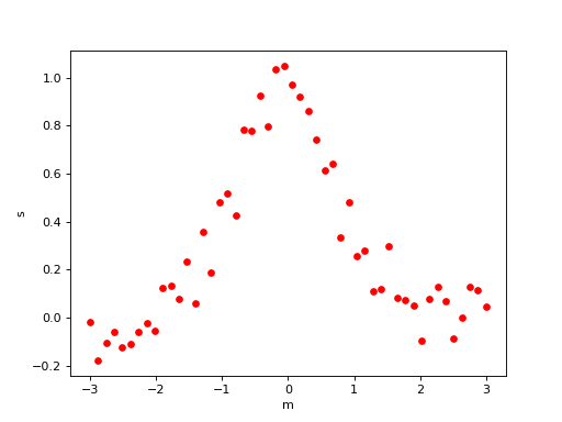
Use the default value for the smoothing parameter:

(Source code, png, hires.png, pdf)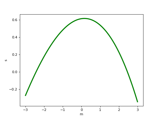

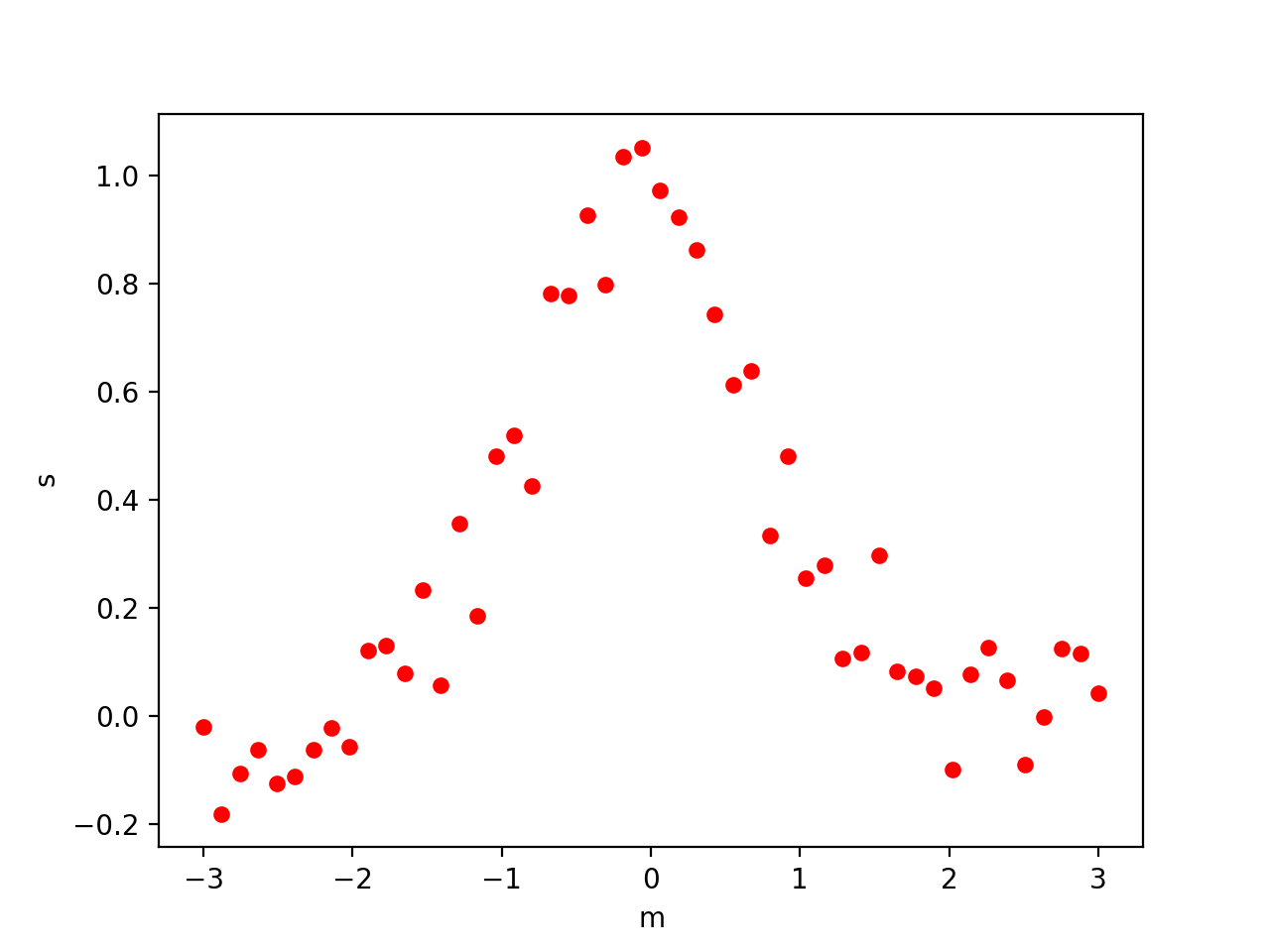
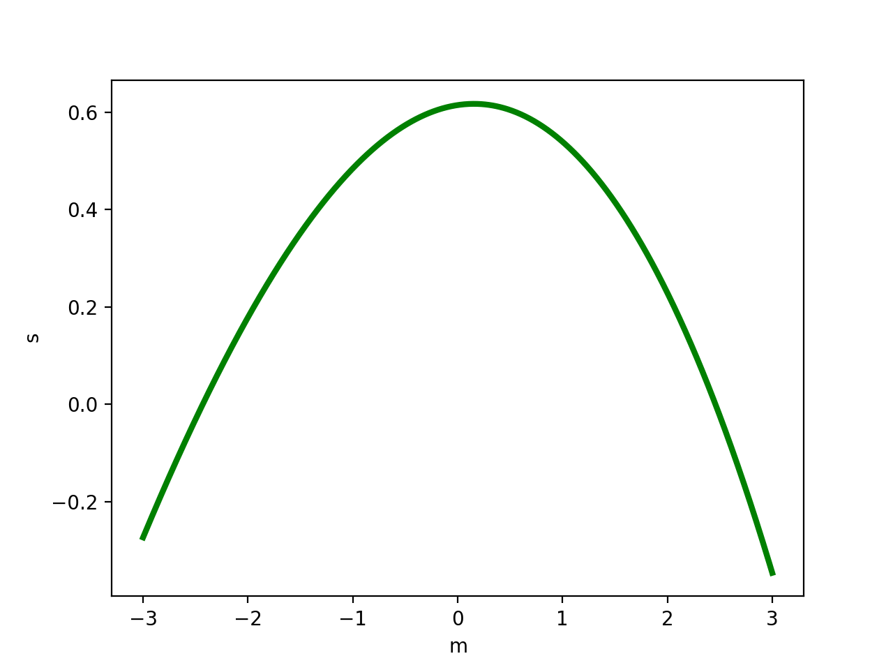
Manually change the amount of smoothing:

(Source code, png, hires.png, pdf)

Attributes Summary

x_unit	Unit of the independent data.
y_unit	Unit of the dependent data.

Methods Summary

__call__(x[, nu, ext])	Evaluate spline (or its nu-th derivative) at positions x.
antiderivative([n])	Construct a new spline representing this spline's antiderivative.
derivative([n])	Construct a new spline representing the derivative of this spline.
derivatives(x)	Return all derivatives of the spline at the point x.
get_coeffs()	Return spline coefficients.
get_knots()	Return positions of interior knots of the spline.
get_residual()	Return weighted sum of squared residuals of spline approximation.
integral(a, b)	Return definite integral of the spline between two given points.
roots()	Return the zeros of the spline.
set_smoothing_factor(s)	Continue spline computation with the given smoothing factor s and with the knots found at the last call.
validate_input(x, y, w, bbox, k, s, ext, ...)

Attributes Documentation

x_unit

Unit of the independent data.

y_unit

Unit of the dependent data.

Methods Documentation

__call__(x: ndarray, nu: int = 0, ext: int | None = None) → Quantity

Evaluate spline (or its nu-th derivative) at positions x.

Parameters:

xndarray or Quantity array_like

A 1-D array of points at which to return the value of the smoothed spline or its derivatives. Note: x can be unordered but the evaluation is more efficient if x is (partially) ordered.

nuint, optional

The order of derivative of the spline to compute.

extint, optional

Controls the value returned for elements of x not in the interval defined by the knot sequence.

• if ext=0 or ‘extrapolate’, return the extrapolated value.

• if ext=1 or ‘zeros’, return 0

• if ext=2 or ‘raise’, raise a ValueError

• if ext=3 or ‘const’, return the boundary value.

The default value is 0, passed from the initialization of UnivariateSpline.

Returns:

yQuantity array_like

Evaluated spline with units y_unit. Same shape as x.

antiderivative(n: int = 1) → USwUType

Construct a new spline representing this spline’s antiderivative.

Parameters:

nint, optional

Order of antiderivative to evaluate. Default: 1

Returns:

splineUnivariateSplinewithUnits

Spline of order k2=k+n representing the antiderivative of this spline.

See also

splantider, derivative

Examples

>>> from scipy.interpolate import UnivariateSpline
>>> x = np.linspace(0, np.pi/2, 70)
>>> y = 1 / np.sqrt(1 - 0.8*np.sin(x)**2)
>>> spl = UnivariateSpline(x, y, s=0)

The derivative is the inverse operation of the antiderivative, although some floating point error accumulates:

>>> spl(1.7) - spl.antiderivative().derivative()(1.7) != 0
True

Antiderivative can be used to evaluate definite integrals:

>>> ispl = spl.antiderivative()
>>> ispl(np.pi/2) - ispl(0)  
2.2572053588768486

This is indeed an approximation to the complete elliptic integral \(K(m) = \\int_0^{\\pi/2} [1 - m\\sin^2 x]^{-1/2} dx\):

>>> from scipy.special import ellipk
>>> ellipk(0.8)  
2.2572053268208538

derivative(n: int = 1) → USwUType

Construct a new spline representing the derivative of this spline.

Parameters:

nint, optional

Order of derivative to evaluate. Default: 1

Returns:

splineUnivariateSpline

Spline of order k2=k-n representing the derivative of this spline.

See also

splder, antiderivative

Examples

This can be used for finding maxima of a curve:

>>> from interpolated_coordinates.utils import UnivariateSplinewithUnits
>>> x = np.linspace(0, 10, 70) * u.s
>>> y = np.sin(x.value) * u.m
>>> spl = UnivariateSplinewithUnits(x, y, k=4, s=0)

Now, differentiate the spline and find the zeros of the derivative. (NB: sproot only works for order 3 splines, so we fit an order 4 spline):

>>> spl.derivative().roots() / np.pi  
<Quantity [0.50000001, 1.5       , 2.49999998] s>

This agrees well with roots \(\\pi/2 + n\\pi\) of \(\\cos(x) = \\sin'(x)\).

derivatives(x: Quantity) → ndarray

Return all derivatives of the spline at the point x.

Parameters:

xQuantity

The point to evaluate the derivatives at.

Returns:

derndarray of Quantity object, shape(k+1,)

Derivatives of the orders 0 to k.

Examples

>>> from scipy.interpolate import UnivariateSpline
>>> x = np.linspace(0, 3, 11)
>>> y = x**2
>>> spl = UnivariateSpline(x, y)
>>> np.round(spl.derivatives(1.5), 2)  
array([2.25, 3.  , 2.  , 0.  ])

get_coeffs() → Quantity

Return spline coefficients.

get_knots() → Quantity

Return positions of interior knots of the spline.

Internally, the knot vector contains 2*k additional boundary knots. Has units of x position

get_residual() → Quantity

Return weighted sum of squared residuals of spline approximation.

This is equivalent to::

sum((w[i] * (y[i]-spl(x[i])))**2, axis=0)

integral(a: Quantity, b: Quantity) → Quantity

Return definite integral of the spline between two given points.

Parameters:

aQuantity

Lower limit of integration.

bQuantity

Upper limit of integration.

Returns:

integralfloat

The value of the definite integral of the spline between limits.

Examples

>>> from scipy.interpolate import UnivariateSpline
>>> x = np.linspace(0, 3, 11)
>>> y = x**2
>>> spl = UnivariateSpline(x, y)
>>> spl.integral(0, 3)
9.0

which agrees with \(\int x^2 dx = x^3 / 3\) between the limits of 0 and 3.

A caveat is that this routine assumes the spline to be zero outside of the data limits:

>>> spl.integral(-1, 4)
9.0

>>> spl.integral(-1, 0)
0.0

roots() → Quantity

Return the zeros of the spline.

Restriction: only cubic splines are supported by fitpack.

set_smoothing_factor(s)

Continue spline computation with the given smoothing factor s and with the knots found at the last call.

This routine modifies the spline in place.

validate_input(x: ndarray | Quantity, y: ndarray | Quantity, w: ndarray | Quantity, bbox: list[Quantity | None], k: int, s: float, ext: int | str, check_finite: float) → tuple[ndarray, ndarray, ndarray, list[Quantity], int | str]